Discontinued...
Sunday, December 22, 2013 2 comments
I have abandoned this blog. No new posts will be made or comments replied to.
Rendering 3D Anaglyph in OpenGL
Sunday, May 29, 2011 3 commentsIt's quite easy (and fun!) to render 3D anaglyphs with OpenGL. I expect you to know what anaglyphs are and how to view them. If not, read this earlier article. The focus of this tutorial is to provide you enough background and code snippets for the task, so that you may have fun rendering anaglyphs with your own programs.
We will focus on producing a red-cyan anaglyph from a given 3D scene. The scene will be rendered twice: Once by setting up the camera for the left eye which will be subsequently filtered to let only red color pass, and other time for the right eye, which will then be filtered so that 'green plus blue' (cyan) components pass. To implement this idea, you'll need to understand the role of parallax in stereoscopic vision and the concept of projection and viewing as they apply to OpenGL. This tutorial assumes familiarity with OpenGL projection and modelview transforms. If you know all that stuff, go on ahead, else just skim through this chapter from the redbook and you'll be prepared.
What is parallax? When you look at a 3D anaglyph without the glasses, you will find that the edges of the objects appear displaced in the red and cyan components of the picture. Observe it in the cylinder below:
 |
| Fig. 1: Sample anaglyph - a cylinder |
The human visual system needs depth cues from a flat image (photograph or display-screen) in terms of how much an object shifts laterally between the left eye and the right eye. When we say parallax, we mean exactly this kind of displacement in the image. To see the effect of parallax in the above image, use red/cyan glasses (red on left eye) and try hovering mouse pointer over the left end of the cylinder. It will look sunken into the screen whereas the front of the cylinder will appear more or less at the same depth as the screen. In rendering an anaglyph, all that we're trying to achieve is to get the right kind of parallax for the objects in the scene and the rest is automatically done in the brain, for free!
Parallax is not just qualitative, it has a numeric value and can be positive, negative or zero. In the application, parallax is created by defining two cameras corresponding to the left and right eyes separated by some distance (called interocular distance or simply eye-separation) and having a plane at a certain depth along the viewing direction (called convergence distance) at which the parallax is zero. Objects at the convergence depth will appear to be at the same depth as the screen. Objects closer to the camera than the convergence distance will seem to be out-of-screen and objects further in depth than the convergence distance will appear inside the screen. Following figure illustrates this situation:
 |
| Fig. 2: Parallax resulting from vertices at different depths |
In this figure, there are two virtual cameras, one for the left eye (with some negative offset from the origin on the X-axis) and the other for the right eye (with some positive offset from the origin on the X-axis). They are separated by the same amount as the offset between human eyes, which averages around 65 mm. Then there is the depth of zero-parallax called convergence depth. You can imagine it as a plane along x-y axes and located at depth of convergence along the negative Z-axis. For illustration of different kinds of parallax three vertices - v1, v2 and v3 are shown.
For each vertex, consider a line from the vertex to each camera and observe where they intersect with the convergence plane. The gap between the points on the convergence plane for left and the right cameras is the measure of parallax generated by the vertex:
- The vertex v1 which is at a greater depth compared to the convergence creates a parallax. Observe that the red and the cyan dots on the convergence plane are oriented the same way as the two cameras: Red dot is towards the left camera and cyan dot is towards the right camera. This is called positive parallax, and the vertex v1 will appear inside the screen upon being rendered.
- The vertex v2 which is at the same depth as the convergence plane creates zero parallax. There are no separate red and cyan points on the convergence plane here, as there were in the previous case. The vertex v2 will appear at the same depth as the screen when rendered.
- The vertex v3, which is located at a distance less than the convergence distance also causes parallax. But the red and cyan points projected on the convergence plane are oriented opposite to the orientation of the cameras. The point corresponding to the left camera is on the right and the point corresponding to the right camera is on the left. This is called negative parallax and the vertex v3 will seem to appear out of the screen when rendered.
Let's look at another anaglyph which illustrates above characteristics of parallax generated by vertices at different depths:
 |
| Fig. 3: Icosahedrons showing negative, zero and positive parallax |
In the figure, there are three icosahedrons. The one the bottom is furthest in the scene and the one at the top is closest to the camera. The icosahedron in the centre is approximately at the same depth as the screen. Notice how the parallax generated for the near and far icosahedrons is of opposite alignment. The closest icosahedron has red edges to the right and cyan edges to the left. This illustrates negative parallax (for glasses with red filter on left eye) and the icosahedron appears slightly out of the screen when viewed from the red-cyan colored glasses. The small icosahedron at the bottom of the figure has red edges to the left and cyan edges to the right. This alignment is same as the colored glasses used to view them. The parallax created is positive and the icosahedron appears inside the screen behind the icosahedron in the centre which is rendered with (almost) no parallax and is at the same depth as the screen.
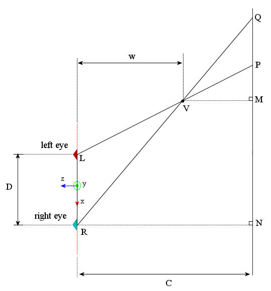
As I mentioned before, parallax can be measured qualitatively. I will now proceed to obtain an equation for parallax introduced in a vertex at a certain depth. While this is not crucially important in setting up the OpenGL for rendering anaglyphs, it is important when you plan the scene and overall range of usable parallax in your interactive application. Consider the following diagram, in which the vertex $V$ is located at depth $w$ and lies beyond the convergence distance:
 |
| Fig. 4: Measuring the amount of parallax for a vertex beyond convergence distance |
The eye separation is $D$ and the convergence distance is $C$. The line joining the left camera $L$ and vertex $V$ meets the convergence plane at $P$. Similarly the line joining the right camera $R$ and the vertex $V$ meets the convergence plane at $Q$. The parallax $p$ associated with the vertex $V$ is the distance $PQ$. Now consider $\Delta LVR$, wherein by use of the intercept theorem we have:\[\frac{PQ}{LR}=\frac{VQ}{VR}\]And by the similarity $\Delta QVM\sim\Delta VRN$, we have \[\frac{VQ}{VR}=\frac{VM}{RN}=\frac{w-C}{w}=1-C/w\]Thus, \[\frac{PQ}{LR}=\frac{p}{D}=1-C/w\]Or\[p=D(1-C/w)\]Similarly for a vertex that is closer than the convergence distance as shown in the figure:
 |
| Fig. 5: Measuring the amount of parallax for a vertex closer than the convergence distance |
The parallax $p$ can be evaluated again by applying the intercept theorem:\[\frac{PQ}{LR}=\frac{QV}{VR}=\frac{QV}{QR-QV}=\frac{\frac{QV}{QR}}{1-\frac{QV}{QR}} \]Now in $\Delta QNR$ since $VM\parallel RN$, we have \[\frac{QV}{QR}=\frac{VM}{RN}=\frac{C-w}{C}=1-w/C\]Thus, \[\frac{PQ}{LR}=\frac{p}{D}=\frac{1-w/C}{w/C}=C/w-1\]Or,\[p=-D(1-C/w)\]
This equation is the same as that for a vertex further than the convergence distance, with a negative sign. The negative sign implies that the projections of the vertex are on the convergence plane are on opposite side as the corresponding camera. If we disregard the sign in the equation, a negative parallax can be understood as the vertex being closer than the convergence distance. A plot of $p=D(1-C/w)$ is shown below:
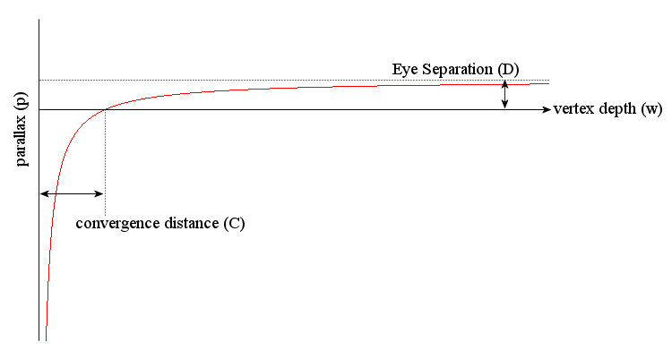 |
| Fig. 6: Variation of parallax with vertex depth for a given convergence distance and eye-separation |
The graph shows that as the vertex moves further and further into the scene, the parallax generated asymptotically approaches the value of eye separation $D$. The parallax remains positive at all vertex depths greater than the convergence distance $C$, at which the parallax is zero. For vertices that are closer in the scene that the distance $C$, the parallax is negative and quickly approaches $-\infty$. Note that for a vertex at $w=C/2$, the parallax obtained is the same as eye separation. Such large vales of negative parallax can make the viewer's eyes diverge causing strain and should be avoided. The practical value of convergence depth is chosen on the basis of the shot being prepared and the type of effect (out of the screen or inside screen) used. Eye separation is typically kept at $1/30^{th}$ of the convergence distance and objects closer than half the convergence distance are avoided in the scene.
The only remaining task is to discuss how we set up a twin camera in OpenGL. In non-stereo mode, you require only one camera, whose viewing parameters are defined by calling glFrustum() or gluPerspective(). The frustum obtained looks like the following:
 |
| Fig. 7(a): A mono frustum |
 |
| Fig. 7(b): Mono frustum (orthographic view from top) |
 |
| Fig. 8(a): Twin-camera system for stereoscopic rendering |
In this setup, we have two frustums: One originating at point $L$ (for the left eye) and the other originating at point $R$ (for the right eye). The distance $LR$ is the eye-separation, so that the points $L$ and $R$ are offset from the origin along negative and the positive X-axes respectively by an amount $\frac{LR}{2}$ each. Observant readers might have already noticed that the the two frustums in the figure above are not the same as the mono-frustum that was shown before and that we did not offset a mono-frustum along the X-axis to obtain the twin-camera system. In fact, the two frustums shown above are asymmetric, whereas the mono-frustum was symmetric (see the next two figures for a better idea). If the two frustums were symmetric and displaced laterally, they wouldn't converge at all. Asymmetry causes the two frustums to converge at the convergence distance. The magenta colored rectangle at the convergence distance represents the virtual screen for the stereoscopic rendering. Any vertex at on the virtual screen will be appear with zero-parallax. Vertices closer or further than this distance will cause appropriate amounts of negative or positive parallax. Following figure shows the same system with an orthographic view from top:
 |
| Fig. 8(b): Stereo-frustum (orthographic view from top) |
The asymmetry of the frustums is clearly evident above. Also notice that the view direction for each frustum is parallel to the other and also to the the Z-axis, same as would be for a mono-frustum. This is the correct way to set-up the stereo pair. There is another twin-camera setup method called toed-in cameras that involves symmetric frustums but the left and right view directions are at an angle to each other. It is sufficient to say that toed-in camera setup is incorrect. Here's another figure showing our stereo-camera system along the Z-axis:
 |
| Fig. 8(c): Stereo-frustum (orthographic view from back) |
At this point we know sufficiently to calculate the stereoscopic frustum parameters which we can use in an OpenGL program. Observe the following figure:
 |
| Fig.9: Calculation of frustum parameters |
While it appears formidable, no new information has been added to the figure above. If you have understood everything so far, you will breeze through the simple calculations that follow. We have, as before, two cameras located at points $L$ and $R$ on the X-axis. The separation $LR$ between them is $D_eye$ and their offsets are symmetric about the origin. The camera directions are parallel, both looking down $-Z$ axis. The near clipping distance of the frustums is $D_{near}$ and the convergence distance is $C$. The extremities of the virtual screen are at points $A$ and $B$ as seen in the top-view. Point $A$ is where the left side of both frustums meet and point $B$ is where the right side of both frustums meet.
In OpenGL, the only way to create an asymmetric frustum is through the glFrustum(). The function gluPerspective() creates only symmetric frustums and hence cannot be used in this case. gluPerspective() takes natural looking parameters such as the field of view angle along Y-direction $\theta_{FOV_{Y}}$ (see fig. 7(a)), the aspect ratio and the distance of the near and far clipping planes. For glFrustum(), you need to provide near clipping plane's top, bottom, left and right coordinates, as well as the distance of the near and far clipping planes. We will compute these parameters from the geometry of the dual frustum shown above.
In the figure, the equivalent of a mono-frustum corresponding to the virtual screen would be $AOB$. Let its field of view along $Y$ direction be $\theta_{FOV_{Y}}$ and the aspect ratio be $r_{aspect}$ (same way these are in gluPerspective()). Then the $top$ and $bottom$ parameters for the glFrustum() will evaluate as:\[top=D_{near} tan\frac{\theta_{FOV_{Y}}}{2}\]\[bottom=-top\] These values apply to both left and right frustums. The half-width $a$ of the virtual screen is\[a=r_{aspect}Ctan\frac{\theta_{FOV_{Y}}}{2}\] Now look at the left frustum $ALB$. The near clipping plane intersects it at $d_{left}$ distance left of $LL'$ and $d_{right}$ distance right of $LL'$. In $\Delta ALL'$ and $\Delta BLL'$, \[\frac{d_{left}}{b}=\frac{d_{right}}{c}=\frac{D_{near}}{C}\]Also, we have\[b=a-\frac{D_{eye}}{2}\]\[c=a+\frac{D_{eye}}{2}\]So that we can readily calculate $d_{left}$ and $d_{right}$. Similarly for the right frustum $ARB$, we could obtain $d_{left}$ and $d_{right}$ by interchanging $b$ and $c$. Here is a code snippet showing how you could wrap the above equations in a small class called StereoCamera:
The code does exactly what we described with the equations and diagrams earlier. Once you have created a StereoCamera object, you can call the methods ApplyLeftFrustum() and ApplyRightFrustum() to set up the respective asymmetric frustums. Note that in these methods, the projection transform is followed by a modelview transform in which we translate along the X-axis. This has the effect of moving the camera to a position offset from the origin. As such there is no camera transform in OpenGL. What we do is move the world in a direction opposite to the conceptual camera using the modelview transform. In order to use the above class, you could write your OpenGL rendering function as the following:
We begin the rendering function by clearing the color and depth buffers. Then we set up the stereo camera system. We apply the left frustum and instruct OpenGL to allow only red components in the color buffer. Then we call the routine to draw the scene. After this we clear the depth buffer, but retain the color buffer (which has only red-channel values). With depth buffer cleared we activate the right frustum and instruct OpenGL to allow only green and blue color components in the color buffer. We call our drawing routine one more time. Note that the colors scene for the left eye and the scene for the right eye have no overlapping color spaces, so no explicit blending/accumulation is required. Finally we enable all the color channels and the scene gets rendered as anaglyph. Note that we had to render geometry twice. That means that the frame-rate gets reduced to half of what we would obtain with a mono-frustum. This is typical of stereoscopic rendering. If you're wondering what output is generated by the above snippets, here it is:
I will leave you with a video that I made during writing of this (somewhat lengthy) tutorial. The video uses the same theory and code that I covered above. Try to watch this one at 720p full-screen for best effect:
Further Reading:
class StereoCamera
{
public:
    StereoCamera(
        float Convergence,
        float EyeSeparation,
        float AspectRatio,
        float FOV,
        float NearClippingDistance,
        float FarClippingDistance
        )
    {
        mConvergence            = Convergence;
        mEyeSeparation          = EyeSeparation;
        mAspectRatio            = AspectRatio;
        mFOV                    = FOV * PI / 180.0f;
        mNearClippingDistance   = NearClippingDistance;
        mFarClippingDistance    = FarClippingDistance;
    }

    void ApplyLeftFrustum()
    {
        float top, bottom, left, right;

        top     = mNearClippingDistance * tan(mFOV/2);
        bottom  = -top;

        float a = mAspectRatio * tan(mFOV/2) * mConvergence;

        float b = a - mEyeSeparation/2;
        float c = a + mEyeSeparation/2;

        left    = -b * mNearClippingDistance/mConvergence;
        right   =  c * mNearClippingDistance/mConvergence;

        // Set the Projection Matrix
        glMatrixMode(GL_PROJECTION);
        glLoadIdentity();
        glFrustum(left, right, bottom, top,
                  mNearClippingDistance, mFarClippingDistance);

        // Displace the world to right
        glMatrixMode(GL_MODELVIEW);
        glLoadIdentity();
        glTranslatef(mEyeSeparation/2, 0.0f, 0.0f);
    }

    void ApplyRightFrustum()
    {
        float top, bottom, left, right;

        top     = mNearClippingDistance * tan(mFOV/2);
        bottom  = -top;

        float a = mAspectRatio * tan(mFOV/2) * mConvergence;

        float b = a - mEyeSeparation/2;
        float c = a + mEyeSeparation/2;

        left    =  -c * mNearClippingDistance/mConvergence;
        right   =   b * mNearClippingDistance/mConvergence;

        // Set the Projection Matrix
        glMatrixMode(GL_PROJECTION);
        glLoadIdentity();
        glFrustum(left, right, bottom, top,
                  mNearClippingDistance, mFarClippingDistance);

        // Displace the world to left
        glMatrixMode(GL_MODELVIEW);
        glLoadIdentity();
        glTranslatef(-mEyeSeparation/2, 0.0f, 0.0f);
    }

private:
    float mConvergence;
    float mEyeSeparation;
    float mAspectRatio;
    float mFOV;
    float mNearClippingDistance;
    float mFarClippingDistance;

};
The code does exactly what we described with the equations and diagrams earlier. Once you have created a StereoCamera object, you can call the methods ApplyLeftFrustum() and ApplyRightFrustum() to set up the respective asymmetric frustums. Note that in these methods, the projection transform is followed by a modelview transform in which we translate along the X-axis. This has the effect of moving the camera to a position offset from the origin. As such there is no camera transform in OpenGL. What we do is move the world in a direction opposite to the conceptual camera using the modelview transform. In order to use the above class, you could write your OpenGL rendering function as the following:
// main rendering function
void DrawGLScene(GLvoid)
{
    glClear(GL_COLOR_BUFFER_BIT | GL_DEPTH_BUFFER_BIT);

    // Set up the stereo camera system
    StereoCamera cam(
        2000.0f,     // Convergence
        35.0f,       // Eye Separation
        1.3333f,     // Aspect Ratio
        45.0f,       // FOV along Y in degrees
        10.0f,       // Near Clipping Distance
        20000.0f);   // Far Clipping Distance

    cam.ApplyLeftFrustum();
    glColorMask(true, false, false, false);

    PlaceSceneElements();

    glClear(GL_DEPTH_BUFFER_BIT) ;

    cam.ApplyRightFrustum();
    glColorMask(false, true, true, false);

    PlaceSceneElements();

    glColorMask(true, true, true, true);
}


void PlaceSceneElements()
{
    // translate to appropriate depth along -Z
    glTranslatef(0.0f, 0.0f, -1800.0f);

    // rotate the scene for viewing
    glRotatef(-60.0f, 1.0f, 0.0f, 0.0f);
    glRotatef(-45.0f, 0.0f, 0.0f, 1.0f);

    // draw intersecting tori
    glPushMatrix();
        glTranslatef(0.0f, 0.0f, 240.0f);
        glRotatef(90.0f, 1.0f, 0.0f, 0.0f);
        glColor3f(0.2, 0.2, 0.6);
        glutSolidTorus(40, 200, 20, 30);
        glColor3f(0.7f, 0.7f, 0.7f);
        glutWireTorus(40, 200, 20, 30);
    glPopMatrix();

    glPushMatrix();
        glTranslatef(240.0f, 0.0f, 240.0f);
        glColor3f(0.2, 0.2, 0.6);
        glutSolidTorus(40, 200, 20, 30);
        glColor3f(0.7f, 0.7f, 0.7f);
        glutWireTorus(40, 200, 20, 30);
    glPopMatrix();
}
We begin the rendering function by clearing the color and depth buffers. Then we set up the stereo camera system. We apply the left frustum and instruct OpenGL to allow only red components in the color buffer. Then we call the routine to draw the scene. After this we clear the depth buffer, but retain the color buffer (which has only red-channel values). With depth buffer cleared we activate the right frustum and instruct OpenGL to allow only green and blue color components in the color buffer. We call our drawing routine one more time. Note that the colors scene for the left eye and the scene for the right eye have no overlapping color spaces, so no explicit blending/accumulation is required. Finally we enable all the color channels and the scene gets rendered as anaglyph. Note that we had to render geometry twice. That means that the frame-rate gets reduced to half of what we would obtain with a mono-frustum. This is typical of stereoscopic rendering. If you're wondering what output is generated by the above snippets, here it is:
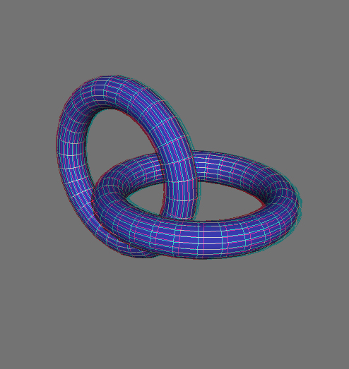 |
| Fig. 10: Output of the drawing routine in the listing above |
I will leave you with a video that I made during writing of this (somewhat lengthy) tutorial. The video uses the same theory and code that I covered above. Try to watch this one at 720p full-screen for best effect:
Further Reading:
You could find a lot of material on stereographics compiled by Paul Bourke on this page. You can also watch a video presentation by NVIDIA from GTC 2010 here and download the slides for offline viewing.
Have fun!
Poor man's stereo 3D
Sunday, April 17, 2011 2 comments
The red/cyan anaglyphs have been around for decades now and they are still the most inexpensive ways to experience 3D. The idea is to capture a scene from two different points of view (by keeping the same kind of gap between the cameras as the human eyes) and then filter the left and right eye images through red and cyan filters. Finally the two scenes are superimposed on a screen or paper/film.
To be able to view these images, one needs glasses that can separate the two color components for each eyes as they were originally captured by that special camera arrangement. The glasses too, as you would have guessed, use the same color filters - red and cyan and the human mind is pleasantly befooled into perceiving depth in the scene (hence the sensation of 3D).
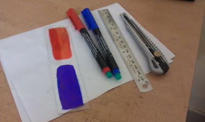
If you ever came across videos and pictures on the web that are anaglyphs and you did not have the means to view them right away, you may just follow the instructions here to make a pair of those glasses for yourself. Being lazy and shameless I made mine using transparent sheets of plastic and red/blue markers:
Once you are done, have a go at this flickr pool dedicated to anaglyph photographs. Youtube also has many 3D anaglyph videos. I watched whole of this video and believe me it was awesome.
As a closing note, don't let yourself believe that the approach described here is the only way you could view stereo-3D images. Vendors are already selling stereo-3D enabled products for some time now and if you need somewhat sophisticated (and less parsimonious) solution, you could definitely go buy them.
To be able to view these images, one needs glasses that can separate the two color components for each eyes as they were originally captured by that special camera arrangement. The glasses too, as you would have guessed, use the same color filters - red and cyan and the human mind is pleasantly befooled into perceiving depth in the scene (hence the sensation of 3D).
If you ever came across videos and pictures on the web that are anaglyphs and you did not have the means to view them right away, you may just follow the instructions here to make a pair of those glasses for yourself. Being lazy and shameless I made mine using transparent sheets of plastic and red/blue markers:

Once you are done, have a go at this flickr pool dedicated to anaglyph photographs. Youtube also has many 3D anaglyph videos. I watched whole of this video and believe me it was awesome.
As a closing note, don't let yourself believe that the approach described here is the only way you could view stereo-3D images. Vendors are already selling stereo-3D enabled products for some time now and if you need somewhat sophisticated (and less parsimonious) solution, you could definitely go buy them.
Trying out the ARToolkit
Sunday, September 5, 2010 3 commentsARToolkit provides a simple framework to build your own augmented reality applications. Acquisition of video frames and identification of markers is built-in so that you can directly obtain the camera transformation relative to the detected patterns. I was looking for ways to register interactive input in my 6 DOF inverse kinematic solver that I wrote earlier (I wish to write a tutorial on the inverse kinematic solver as well but at the moment typing in all the math seems intimidating). So far I have succeeded in making an overlay of the manipulator arm on the live video relative to the marker. Maybe I will be able to do some pick and place kind of stuff with this thing soon... stay tuned.
 |
| The 6 DOF manipulator in the AR environment - my table-top :) |
Making a USB based AVR Programmer
Monday, March 29, 2010 26 commentsAround time when I was beginning to learn about microcontrollers I had exchanged my laptop with a senior at college for his desktop - that's because the only way I knew how to program an ATMEGA chip was through either a serial port or a parallel port. USB programmers were not available widely and were generally thought to be expensive. The programming setup using a parallel port was very simple. I followed the DAPA programmer for my needs for some time. Here is a pic of the setup - ATMEGA8 chip on breadboard (pinouts matched against the one shown in above link), a parallel port DB25 connector and a USB cable that just to get 5V and GND quick and dirtly without any batteries and voltage regulators:

Over the time I learned about an inexpensive way of making a USB based AVR programmer called USBasp. It's faster, cheaper and has the convenience of letting you program AVRs from laptops. Here is a pic of the first USBasp programmer that I built, and promptly got my laptop back (in the link you can see more designs):

Plugging it into the laptop and seeing it get recognized was pure fun! Having it work right also meant that you could get it to a competition venue easily, in case you had to program the microcontroller again. Without this the only other way was to bring along a desktop which was just impractical. I can recall once at the IIT Techfest I had found a team bring a really old laptop which did have a parallel port and those folks were programming their chips on the spot and it just didn't feel fair for the rest of us... heh heh! I used this one for a long time, even took it to workshops at college and many came from time to time to get their microcontrollers programmed. Right now the one in the pic is with a friend who is using it for the project work at college. And here is another one that I built yesterday:

Looks neat, doesn't it! But making it wasn't hassle free this time. I started with programming an ATMEGA8 needed for the USBasp with DAPA programmer like the one in the first pic (except for I was not using an external crystal). Having written the USBasp firmware on the chip, I proceeded to program fuses (they need to be done for using the 12 MHz external crystal). One fuse byte got written and then the chip lost sync with the programmer. My programming softwares - both avrdude and uisp complained that they cannot read the chip. Such bad fuse scenarios are common and the one sweet way to recover the chip is to attach a crystal of right value to the dead chip and retry with the programmer. Alas, I did not have any ~20/22/27 pF caps in my stock to use with the crystal. I had to go to the local (which in my case is nowhere nearby) parts shop and I got the wretched caps that cost only two teaspoons of sugar! But then things flowed smoothly, after the dead chip received the much needed CPR and I got that neat looking DIY USB programmer for myself again.
LED Matrix Game
Thursday, August 6, 2009 12 commentsMaking games is cool and making them in hardware with blinking LEDs is cooler still. If you ever wondered how to make an LED matrix game yourself, this article is for you. I have discussed the most basic 8x8 LED matrix based design and the code samples should be adequate to prepare you to write your own game. I assume you have familiarity with Atmel's ATMEGA microcontrollers and that you can follow circuit schematics and assemble the necessary parts yourself. I have not used any ready-made 8x8 modules. The LEDs have been meticulously assembled on a veroboard by wiring and soldering on the back. I have used WinAVR for development and the source code and various snippets are provided in C for the same.
The game system has three parts as shown below:

The user pushes the buttons in order to select menu options and play the game(s). The inputs are interpreted by the microcontroller and the LED matrix display is updated as the game logic dictates. Displaying 8x8 = 64 LEDs simultaneously can be daunting. So lets go step by step. Following schematic shows how you connect a single LED - a staple Hello World!

#include<avr/io.h>
#include<util/delay.h>

int main(void)
{
 DDRA=0xFF;
 while(1)
 {
  PORTA=0X00;
  _delay_ms(200);
  PORTA=0x01;
  _delay_ms(200);
 }
 return(0);
}
This, I guess you already know. A single LED is connected to PORTA PIN0, through a current limiting resistor from anode side and the cathode is made ground. In the program you declare the PORTA pins to be output and then in an infinite loop you make the PIN0 on PORTA go high and low, making the LED blink. Now think for a moment: In an 8x8 matrix there are 64 LEDs. If you are using ATMEGA16/32 you have 40 pins out of which only 32 are IO pins grouped as 4 ports of 8 pins each. So even if you use all the 32 pins in the manner shown above, you are able to light up only 32 LEDs, not the whole matrix. More importantly in doing so you have run out of the pins that you could possibly use for push-button inputs. So how can we overcome this stumbling block? A solution that is found in several designs is as shown below:

Here, LEDs in the same column have the anodes on a common line, running top to bottom. Similarly for LEDs in a single row have cathodes on a common line, running left to right. This means that if on the wires that make up the column an 8 bit pattern say 10111110 is set and then the common line for some row is grounded, then the LEDs in that particular row will glow as dictated by this bit-pattern. With this bit-pattern, for example, if you ground the common line for the topmost row then the LED1 and LED7 will be OFF and rest in that row will be ON. You may ground the common line on any row and the bit-pattern set on the column wires will appear as glowing LEDs in that particular row.
This design, however, is not the complete solution. The reason is that different rows cannot display different bit patterns. They will all display the same pattern that has been set on the column wires, once they are grounded. In order to overcome this problem, we shall use a clever trick - persistence of vision. The idea is that if changes are made in rapid succession, the human eye is unable to sense the small incrementals and perceives the event as smooth continuous motion. In practice we display one row at a time - we set the bit pattern on the column for the topmost row and ground that row keeping all other rows un-grounded. Next, we set the bit pattern for the second row on the column wires and then ground the second row, keeping all other rows un-grounded and so on till we have displayed all the rows, one at a time, in succession from top to bottom. We repeat the same process over and over again, just like scan-lines in a TV. We make the switching between the rows so fast that it appears that you are viewing the entire LED matrix in one go.
Now we can attach the 8x8 LED module shown above to two different ports - one to set bit patterns for the column wires and other to ground different rows when desired. In the following figure PORTC is used to set patterns on column wires and PORTA is used to ground rows:

This type of connection has some drawbacks too. The thing is when a row is grounded then current from all the LEDs that are ON in that row sinks collectively at this pin and this may be dangerous for the microcontroller. That's where the driver IC shown in the figure on the top comes into picture. We use ULN2803 to sink the current safely from all 8 rows. The ULN2803 IC is shown below:

Pin 9 is connected to ground. Pins 1-8 are connected to the PORTA[0:7] which we use to control the selective sinking of the rows. The row [1:8] wires are connected to pins [18:11] so that when PORTA PIN0 is set ON, the row 1 is connected to the ground. So keeping these factors in mind, the block diagram can be modified as:

Which results into the schematic:

If you have understood everything so far, you will prepare the working hardware without any problems. Only programming remains to be done. I just give some examples and explain them:
/* Glow all LEDs */
#include <avr/io.h>
#include <avr/interrupt.h>
#include <stdlib.h>
#include <avr/delay.h>
#include <avr/wdt.h>

unsigned char     matrix[8];  // The matrix that is directly copied to the LEDs
static int      current_row;  // The current row being sinked by 2803 IC
unsigned char    PORTD_Val;


void clearmatrix(){
 for(int i=0; i<8; i++)
  matrix[i] = 0x00;
}

void setpixel(unsigned char *s, int x, int y){
    unsigned char ch;
 ch = *(s+y);
 *(s+y) = (ch | (128>>x));
}


void resetpixel(unsigned char *s, int x, int y){
    unsigned char ch;
 ch = *(s+y);
 *(s+y) = (ch & ~(128>>x));
}

int ispixel(unsigned char *s, int x, int y){
    unsigned char ch;
 ch = *(s+y);
 if((ch & (128>>x))!=0)
  return 1;
 else
  return 0;
}


int main (void)
{
 wdt_disable();

 /* Initialise GPIO */
 DDRA |= 0xFF;
 DDRC |= 0xFF;
 DDRD &= 0x00;      // The port used as input

 PORTA = 0x00;      // No initial value on PORTA
 PORTC = 0x00;      // No initial value on PORTC
 PORTD = 0xFF;      // Enable internal pull up resistors


 /* Initialize timer */
 TCCR1B |= (1 << WGM12);    // Configure timer 1 for CTC mode
 TIMSK  |= (1 << OCIE1A);    // Enable CTC interrupt
 sei();        // Enable global interrupts
 OCR1A   = 3000;      // Set CTC compare value
 TCCR1B |= (1 << CS10);    // Div by 1


 clearmatrix();

 int i, j;

 for (;;)
 {
   for(i=0; i<8; i++)
    for(j=0; j<8; j++)
    {
     setpixel(matrix, i, j);
     _delay_ms(100);
    }

 }
}

ISR(TIMER1_COMPA_vect)
{
 PORTC = matrix[current_row];

 PORTA = 1<<current_row;

 current_row++;

 if (current_row == 8)
  current_row = 0;

}
I maintain a global unsigned char called matrix of 8 bytes. This is the display screen for the rest of the program to use. Clearly 8 bytes means 64 bits representing ON/OFF state of all the LEDs in the matrix. matrix[0] is supposed to mean the top row, matrix[1] the next row and so on till matrix[7] - the row at the bottom.
Another global is current_row to track which row you are supposed to sink current at through ULN2803 IC attached at PORTA. The sinking of the row is timed through TIMER1 ISR shown at the end of the program. This sets the column bits on PORTC based on the current_row value and also makes the appropriate row sink current. This done it cycles through other values of current_row.
With the matrix so defined and the ISR automatically taking care when to update the display, the rest of the program can focus on the application. I have made functions setpixel(), resetpixel(), clearmatrix() and ispixel() which work as if the 8x8 matrix were a graphical screen with top left corner of coordinates (0,0) and x increasing column-wise from 0 to 7 and y increasing from top to bottom row as 0 to 7. The functions are used to turn on, turn off an LED given (x,y), then clear entire matrix and also to inspect whether a particular (x,y) pixel is on or not respectively. You can clearly see how in the main loop we have conveniently made use of setpixel().
The following snippet shows manipulation of a pixel on the matrix. Pressing four keys attached to the microcontroller designated UP, DOWN, LEFT and RIGHT moves a single glowing LED across the display. in response This is the simplest idea that is exploited to make more complete games:
.
.
int main (void)
{
 wdt_disable();

 /* Initialise GPIO */
 DDRA |= 0xFF;
 DDRC |= 0xFF;
 DDRD &= 0x00;      // The port used as input

 PORTA = 0x00;      // No initial value on PORTA
 PORTC = 0x00;      // No initial value on PORTC
 PORTD = 0xFF;      // Enable internal pull up resistors


 /* Initialize timer */
 TCCR1B |= (1 << WGM12);    // Configure timer 1 for CTC mode
 TIMSK  |= (1 << OCIE1A);    // Enable CTC interrupt
 sei();        // Enable global interrupts
 OCR1A   = 3000;      // Set CTC compare value
 TCCR1B |= (1 << CS10);    // Div by 1


 clearmatrix();

 int x=0, y=0;


 for (;;)
 {
  PORTD_Val = PIND;
  if (!(PORTD_Val&(1<<0))) // Detect pushbutton pressed at the pin PORTD0 (left)
   x--;
  if (!(PORTD_Val&(1<<1))) // Detect pushbutton pressed at the pin PORTD1 (right)
   x++;

  if (!(PORTD_Val&(1<<2))) // Detect pushbutton pressed at the pin PORTD2 (up)
   y--;

  if (!(PORTD_Val&(1<<3))) // Detect pushbutton pressed at the pin PORTD3 (down)
   y++;

  // Check range of x and y
  if (x<0) x=0;
  if (x>7) x=7;
  if (y<0) y=0;
  if (y>7) y=7;

  // Draw a pixel with these positions of x and y
  clearmatrix();    // Clear all previously done drawing
  setpixel(matrix, x, y); // Draw at the current x and y location
  _delay_ms(100);

 }
}
.
.
Finally, a word on using fonts. Fonts are just 8x8 bit patterns. You can lay them out on a grid and obtain hexadecimal values for each row and then put them in an array for reference. I once found this 8x8 pixel font editor that you may find interesting. More advanced users may choose to create all the letters of the alphabet and store them on EEPROM. Anyway, here is the snippet that shows how to make fonts and display them:
.
.
//global
unsigned char font_T[8] = {0x7f, 0x49, 0x08, 0x08, 0x08, 0x08, 0x1c, 0x00};
unsigned char font_O[8] = {0x1e, 0x21, 0x21, 0x21, 0x21, 0x21, 0x1e, 0x00};
unsigned char font_M[8] = {0x21, 0x33, 0x2d, 0x21, 0x21, 0x21, 0x21, 0x00};
.
.
.
int main(void)
.
.
 clearmatrix();

 int i;

 for (;;)
 {
  PORTD_Val = PIND;

  if (!(PORTD_Val&(1<<2))) // Detect pushbutton pressed at the pin PORTD2 (show T)
  {
   for(i=0; i<7; i++)
    matrix[i] = font_T[i];
  }

  if (!(PORTD_Val&(1<<1))) // Detect pushbutton pressed at the pin PORTD1 (show O)
  {
   for(i=0; i<7; i++)
    matrix[i] = font_O[i];
  }

  if (!(PORTD_Val&(1<<0))) // Detect pushbutton pressed at the pin PORTD0 (show M)
  {
   for(i=0; i<7; i++)
    matrix[i] = font_M[i];
  }
 }
.
.
I will leave you with a video of the game system I built. This one was made for the college competition with teammates Navneet and Neelav. As you can see I have managed four games and a menu based on scrolling text. I did not cover these in this article. Hope you are able to figure out yourselves :)
Subscribe to:
Posts
(
Atom
)